 Figure
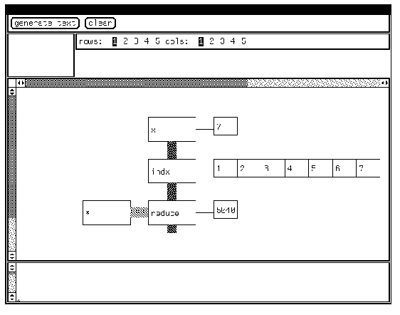
4.1. Factorial calculation.
In the previous chapter we created a simple visual language. In this chapter we use some of the ideas of the simple visual language to create a visual version of APL. We begin with a simple example of the language in use.

We read the diagram vertically, in three stages. In the first stage
a variable x is set to 7. The number 7 is typed in, and can
be edited. In the second stage, the value of x is passed to the
index function, resulting in a vector 1..x, which is displayed as
an intermediate result. In the third state, this vector is reduced by the
multiplication operator, with the final result displayed.
We can compare this to the factorial calculation in the previous chapter,
figure 3.6. The visible difference is the creation of intermediate results
of the calculation. We have also dropped the convention of indicating types
with the fill patterns of the box connectors. Instead, we can perceive
the difference between a scalar, vector, or array by looking at the intermediate
results.
APL operators take either one or two parameters; this allows us to use
the simple graphic representation of the last chapter. Later we will discuss
the ordering of parameters for binary operators.
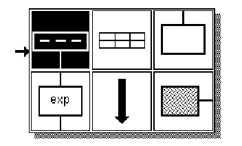
The above figure represents the menu for the objects in the language.
The first box is the primary input box. The second icon represents an array,
which can be attached to the initial box so values can be plugged into
it. The third is an output file box. On the second row, the first icon
represents an expression box. The next icon represents execution; when
this icon is pressed the program will execute. The final icon is a parameter
box.
The normal process of program creation would start by clicking on the
first icon, which would create the initial input variable. The next icon
to be pressed would be the array icon; before doing that it may be necessary
to change the default shape of the array. This is done with the simple
control panel at the top of the application:
Figure
4.3. Row and column panel.
This panel sets the size of the input matrix for the initial value of
the function. When the array icon is selected, a corresponding blank array
will be shown with the number of rows and columns shown in inverted video
above:

This is a blank 2 by 3 array. We can fill in the array with numbers
by moving the mouse into corresponding boxes. If we add a function box
below the input box, we then can invoke the function menu from inside the
box:
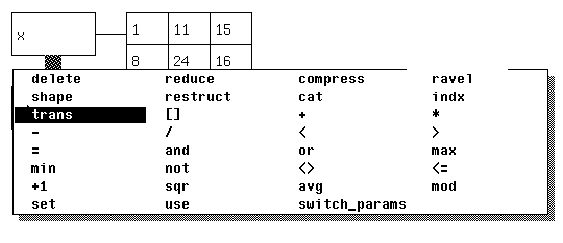
This set of functions includes a set of APL primitives with some additions.
If one of the primitives, such as reduce, is known to take two arguments,
a sideways parameter box will be invoked.
In this case we pick the transpose operator, and execute the program:
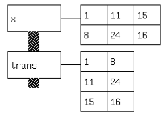
The user creates and fills in the 2 by 3 array. The 3 by 2 array is
generated automatically as part of the execution.
With two-parameter non-commutative functions, it is important to be
able to specify order. The parameter on the left is assumed to be the first
parameter. For example:
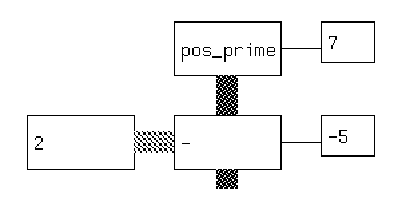
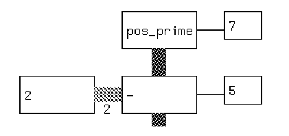
This is equivalent to (2 - 7). If we need (7 - 2), we invoke the function switch_params, which will reverse the order. A 2 appears under the link to the parameter box:
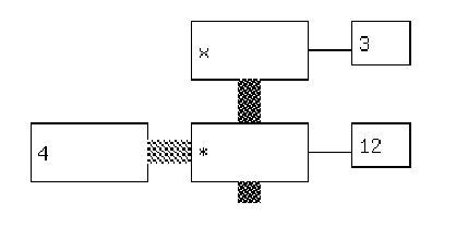
In visual APL, as in APL, we can use an operator such as * on combinations of scalars, vectors, and arrays, with sensible results. We show here (3 * 4):
If we change x to a vector 3 4 5 6 the function returns a vector: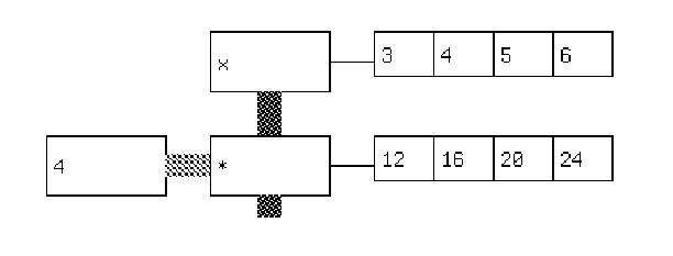
As a more complicated example, operations on arrays often produce vectors.
Reducing a two-dimensional array with multiplication results in a vector
of results, one for each row in the array: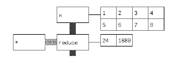
Sometimes it is necessary to set aside a calculation and bring it back
later. In order to accomplish this in a language that is modeled after
a linear string, we need to be able to break the flow and use a previously
calculated variable to start a new stream: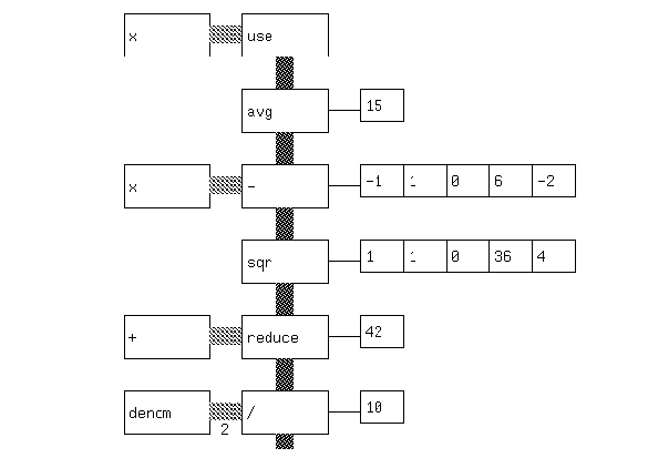
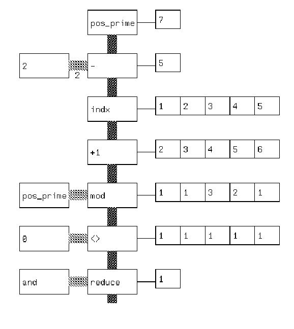
Kamin includes as an example a simple APL-like way of testing for primes.
We include it here as a good example of how a visual front-end can make
some of the concepts of APL clearer. In order to test a prime, we generate
the set of all possible divisors, take the mod of this vector with respect
to the number being tested, and then determine if anything divided evenly.
We present an example where the number is prime, followed by an example
where the number is not prime.
It is probably the case that an experienced APL programmer would not
use this interface to produce code. The experienced programmer gains from
the compactness of the APL symbolic representation. However, even experienced
APL users have problems in reading code not written by themselves; it is
possible that a representation such as the one suggested here would aid
in understanding cryptic one-liner. An APL text representation can be expanded
into a visual APL diagram.
As a teaching tool for novice APL programmers or for students of programming
languages, the work shown here illustrates several concepts in a clear
way. The functional bias of APL is shown by the vertical stream convention
of the overall graph. The concept of functionals is shown by the feeding
of functions into functions as parameters. And the origami-like transformations
of scalars, vectors, and arrays are illustrated through the display of
intermediate results.
For the purposes of interface to an interpreter, every statement results
in a variable called input being set. Code generation for the primality
test follows:
(set input (set pos_prime '( 8)))
(set input (- input 2))
(set input (indx input))
(set input (+1 input))
(set input (mod pos_prime input))
(set input (<> 0 input))
(set input ( and/ input ))
It is also possible to generate a single APL function:
(and/ (<> 0 (mod n (+1 (indx (-n 2))))))
Logistically, the former code generation allows a simple interface into
the interpreter that will return a series of partial results usable in
the display.
The program is coded in C. The user interface is coded in Sunview. The
APL interpreter comes from Kamin (1990). The APL interpreter was modified
in the following ways - it was modified into a subroutine rather than a
main program, and traps were put in to capture results in a vector of arrays
that are returned to the calling program. This vector is used to generate
the data traces which are part of the visual display.
APL itself has a fairly visual, immediate feel. APL2 (J. A. Brown 1988)
incorporates some visualization ideas so that nested data structures can
be viewed and understood. Spreadsheets inspired the concept of editable
array cells; an article by Ambler (1990) discusses extending spreadsheets
to a more abstract level.